Introduction

Package survxai contains functions for creating a unified representation of a survival models. Such representations can be further processed by various survival explainers. Tools implemented in survxai help to understand how input variables are used in the model and what impact do they have on final model prediction.

The analyses carried out using this package can be divided into two parts: local analyses of new observations and global analyses showing the structures of survival models. This vignette describes local explanations.

Methods and functions in survxai package are based on DALEX package.

Use case - data

Data set

In our use case we will use the data from the Mayo Clinic trial in primary biliary cirrhosis (PBC) of the liver conducted between 1974 and 1984. A total of 424 PBC patients, referred to Mayo Clinic during that ten-year interval, met eligibility criteria for the randomized placebo controlled trial of the drug D-penicillamine. The first 312 cases in the data set participated in the randomized trial and contain largely complete data. The pbc data is included in the randomForestSRC package.

data(pbc, package = "randomForestSRC")
pbc <- pbc[complete.cases(pbc),]

head(pbc)

##   days status treatment   age sex ascites hepatom spiders edema bili chol
## 1  400      1         1 21464   1       1       1       1   1.0 14.5  261
## 2 4500      0         1 20617   1       0       1       1   0.0  1.1  302
## 3 1012      1         1 25594   0       0       0       0   0.5  1.4  176
## 4 1925      1         1 19994   1       0       1       1   0.5  1.8  244
## 5 1504      0         2 13918   1       0       1       1   0.0  3.4  279
## 7 1832      0         2 20284   1       0       1       0   0.0  1.0  322
##   albumin copper    alk   sgot trig platelet prothrombin stage
## 1    2.60    156 1718.0 137.95  172      190        12.2     4
## 2    4.14     54 7394.8 113.52   88      221        10.6     3
## 3    3.48    210  516.0  96.10   55      151        12.0     4
## 4    2.54     64 6121.8  60.63   92      183        10.3     4
## 5    3.53    143  671.0 113.15   72      136        10.9     3
## 7    4.09     52  824.0  60.45  213      204         9.7     3

Our original data set contains only the numerical variables. For this usecase we convert variables sex and stage to factor variables.

pbc$sex <- as.factor(pbc$sex)
pbc$stage <- as.factor(pbc$stage)

Models

We will create Cox proportional hazards model based on five variables from our data set: age, treatment, status, sex and bili.

set.seed(1024)
library(rms)
library(survxai)

pbc_smaller <- pbc[,c("days", "status", "treatment", "sex", "age", "bili", "stage")]
head(pbc_smaller)

##   days status treatment sex   age bili stage
## 1  400      1         1   1 21464 14.5     4
## 2 4500      0         1   1 20617  1.1     3
## 3 1012      1         1   0 25594  1.4     4
## 4 1925      1         1   1 19994  1.8     4
## 5 1504      0         2   1 13918  3.4     3
## 7 1832      0         2   1 20284  1.0     3

cph_model <- cph(Surv(days/365, status)~. , data = pbc_smaller, surv = TRUE, x = TRUE, y=TRUE)

Local explanations

In this section we will focus on the local explanations - the explanations for chosen new observations.

Explainers

First, we have to create survival explainers - objects to wrap-up the black-box model with meta-data. Explainers unify model interfacing.

We have to define custom predict function which takes three arguments: model, data and vector with time points. Predict funcions may vary depending on the model. Examples for some models are in Explainations of different survival models vignette.

predict_times <- function(model, data, times){
  prob <- rms::survest(model, data, times = times)$surv
  return(prob)
}

surve_cph <- explain(model = cph_model,
                  data = pbc_smaller[,-c(1,2)], y = Surv(pbc_smaller$days/365, pbc_smaller$status),
                  predict_function = predict_times)

print(surve_cph)

## Model label:  coxph 
## Model class:  cph,rms,coxph 
## Data head  :
##   treatment sex   age bili stage
## 1         1   1 21464 14.5     4
## 2         1   1 20617  1.1     3

Ceteris paribus

Ceteris Paribus Plots (What-If Plots) are designed to present model responses around a single point in the feature space. For more details for generalised models of machine learning see: https://github.com/pbiecek/ceterisParibus.

Ceteris Paribus Plots for survival models are survival curves around one observation. Each curve represent observation with different value of chosen variable. For factor variables curves covers all possible values, for numeric variables values are divided into quantiles.

Ceteris Paribus Plot illustrates how will the survival curve change along with the changing variable.

Below, we plot Ceteris Paribus for one observation.

single_observation <- pbc_smaller[1,-c(1,2)]
single_observation

##   treatment sex   age bili stage
## 1         1   1 21464 14.5     4

cp_cph <- ceteris_paribus(surve_cph, single_observation)
print(cp_cph)

##       y_hat new_x     vname   x_quant quant relative_quant label      time
## 1 0.9789502     1 treatment 0.4927536     0     -0.4927536 coxph 0.1123288
## 2 0.9574511     1 treatment 0.4927536     0     -0.4927536 coxph 0.1397260
## 3 0.9360096     1 treatment 0.4927536     0     -0.4927536 coxph 0.1945205
## 4 0.9147630     1 treatment 0.4927536     0     -0.4927536 coxph 0.2109589
## 5 0.8929362     1 treatment 0.4927536     0     -0.4927536 coxph 0.3013699
## 6 0.8715713     1 treatment 0.4927536     0     -0.4927536 coxph 0.3589041
##     class
## 1 numeric
## 2 numeric
## 3 numeric
## 4 numeric
## 5 numeric
## 6 numeric

After creating the surv_ceteris_paribus object we can visualize it in a very convinient way using the generic plot() function. Black line represent prediction of original observation.

plot(cp_cph, scale_type = "gradient", scale_col = c("red", "blue"), ncol = 2)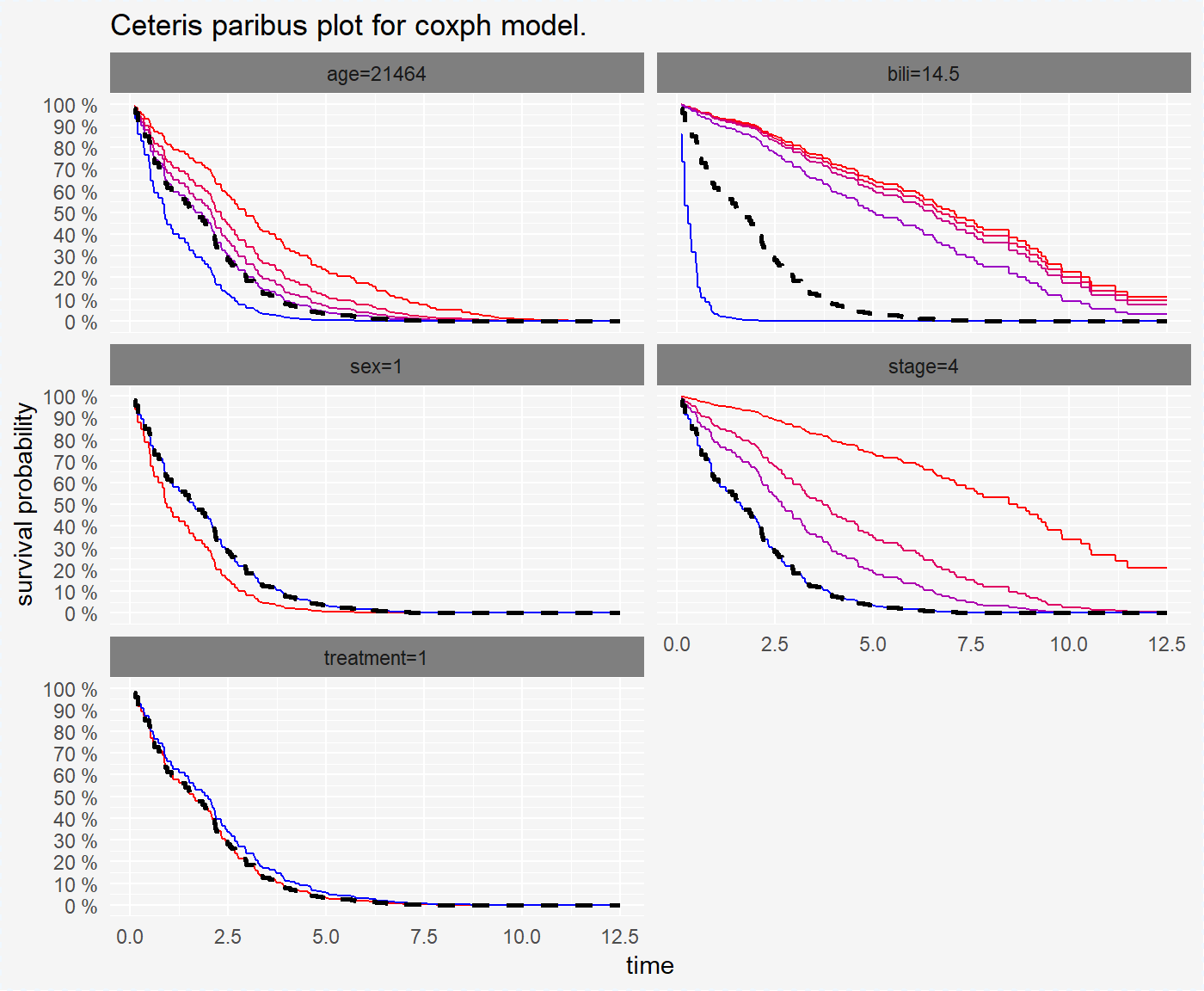

We can see that there are differences for stages. Next, we will plot Ceteris Paribus for sigle variable stage.

plot(cp_cph, selected_variable = "stage", scale_type = "gradient", scale_col = c("red", "blue"))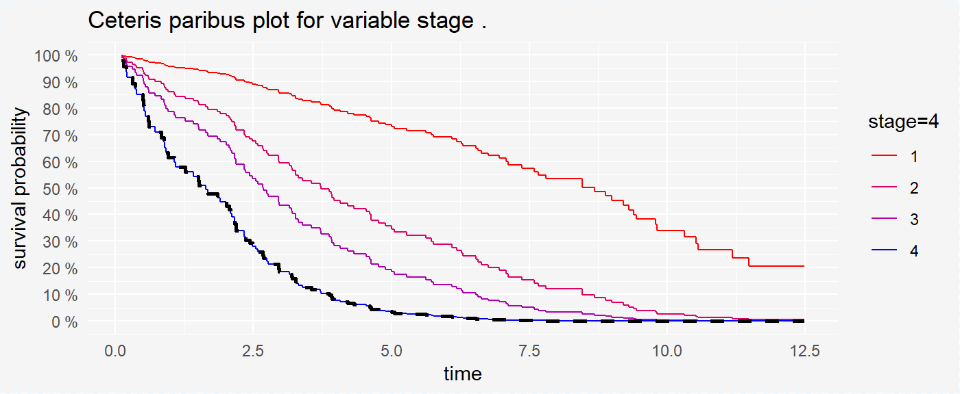

We see a trend that a lower stage means a higher probability of survival for chosen observation.

Prediction breakdown

Break Down Plot presents variable contributions in final predictions. For more details for generalised models of machine learning see: https://github.com/pbiecek/breakDown.

Break Down Plots for survival models compare differences in predictions for median of time.

broken_prediction_cph <- prediction_breakdown(surve_cph, pbc_smaller[1,-c(1,2)])
print(broken_prediction_cph)

##           contribution
## bili          -42.553%
## stage         -19.083%
## age            -5.153%
## treatment      -1.055%
## sex             0.354%

After creating the surv_prediction_breakdown object we can visualize it in a very convinient way using the generic plot() function.

plot(broken_prediction_cph, scale_col = c("red", "blue"))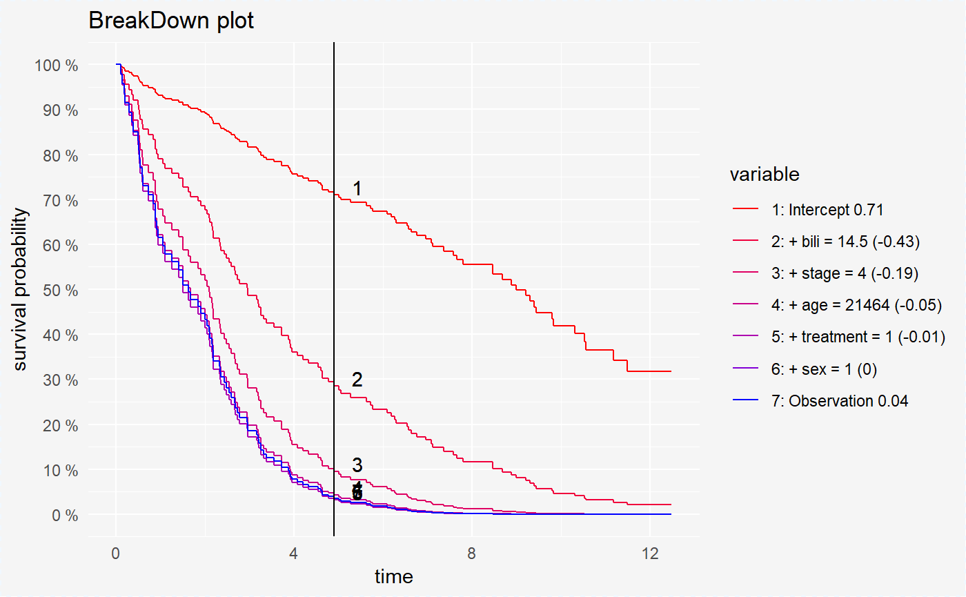

This plot helps to understand the factors that drive survival probability for a single observation.

Survival models - local explanations

Aleksandra Grudziaz

2018-08-20